Interpretability and Shapley Values
Written by James Camp and Jacob Collier
Motivation
Deep Learning/Machine Learning (DL/ML) is increasingly embedded in critical domains like healthcare, finance, law, policing, and more. Models often achieve impressive predictive accuracy, yet for real-world adoption we also need Trust & Transparency. Simply put, stakeholders must understand why an ML model outputs a particular decision.
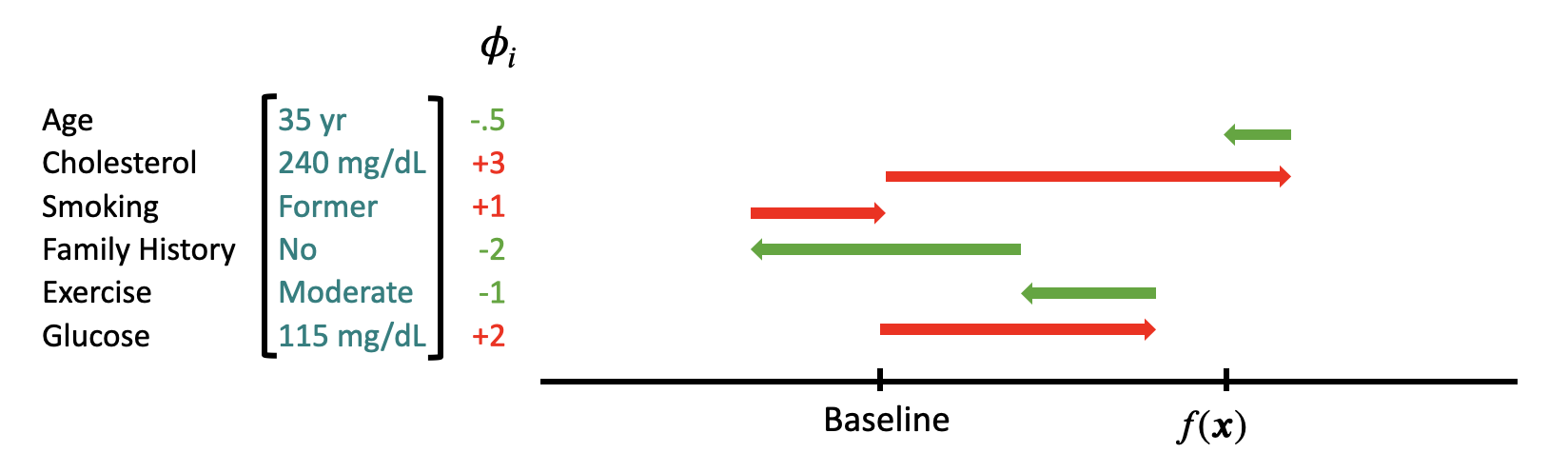
While some simpler models (like linear regression) are intrinsically interpretable, state-of-the-art models (like deep neural networks) appear, to us, as “black boxes,” meaning we have a hard time understanding why they make the predictions they do. Shapley values provide a formal, axiom-based framework for attributing a model’s prediction to its input features, helping to (hopefully) allow us to get a better understanding of what’s going on within the “black box.”
Shapley Value
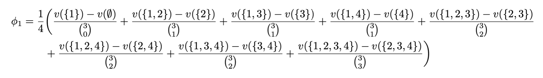
We define the Shapley value for feature (i) as:
\[ \phi_i = \frac{1}{n} \sum_{S \subseteq [n] \setminus \{i\}} \frac{v\bigl(S \cup \{i\}\bigr) - v(S)}{\binom{n-1}{|S|}}. \]
The average over all sizes (k) of the average over sets of size (k):
\[ \phi_i = \frac{1}{n} \sum_{k=0}^{n-1} \frac{1}{\binom{n-1}{k}} \sum_{\substack{S \subseteq [n] \setminus \{i\}:|S|=k}} \bigl(v(S \cup \{i\}) - v(S)\bigr). \]
Let’s try computing some Shapley Values:
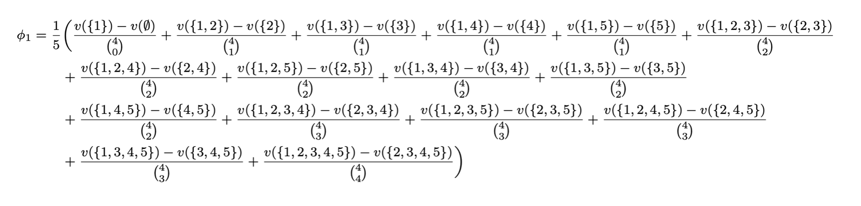
Case (i=1) and (n=4):
Case (i=1) and (n=5):
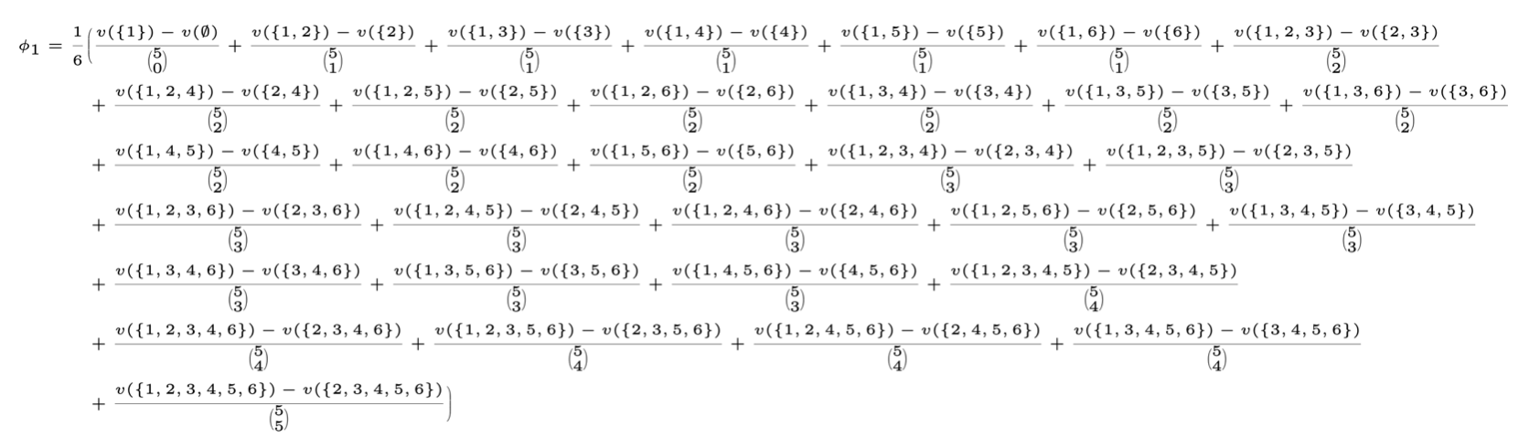
Case (i=1) and (n=6):
Observation
Directly computing all these terms is \(O(2^n)\) quickly becomes infeasible for large n.
Key question: How do we efficiently compute Shapley values without enumerating all \(2^n\) subsets?
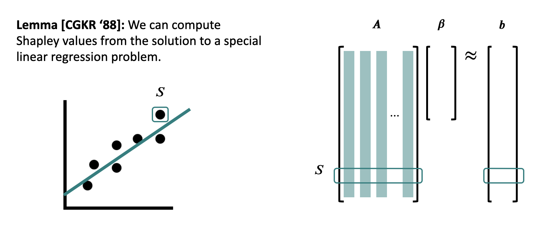
Regression Formulation
Rather than computing every Shapley value, it is possible to use linear regression to approximate them, however this still has some issues:
Linear regression is unable to effectively approximate non-linear relations. That is to say in the case that the Shapley values are highly non-linear then a regression formulation is unlikely to be able to be accurate.
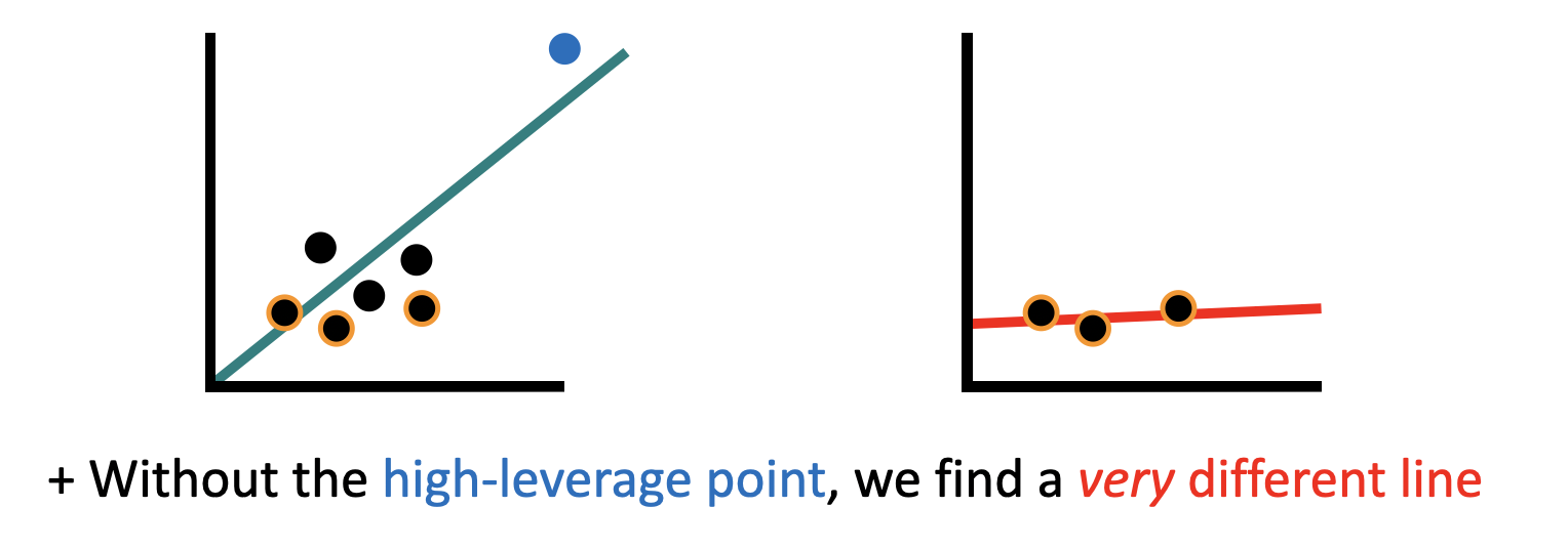
Linear regression can also struggle to cope with significant data outliers.
In order to train this regression model we are already calculating the Shapley values, resulting in \(O(2^n)\) time complexity.
Kernel Shap
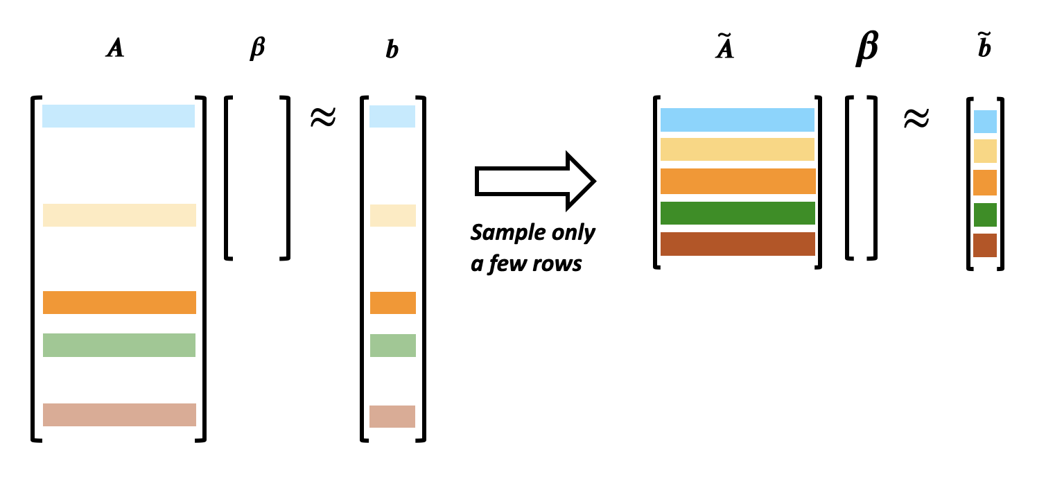
Motivation: The \(O(2^n)\) time complexity leads to poor scaling, and results in infeasibility for most neural networks, however by using linear regression on only a subset of the inputs we are able to reduce the complexity.
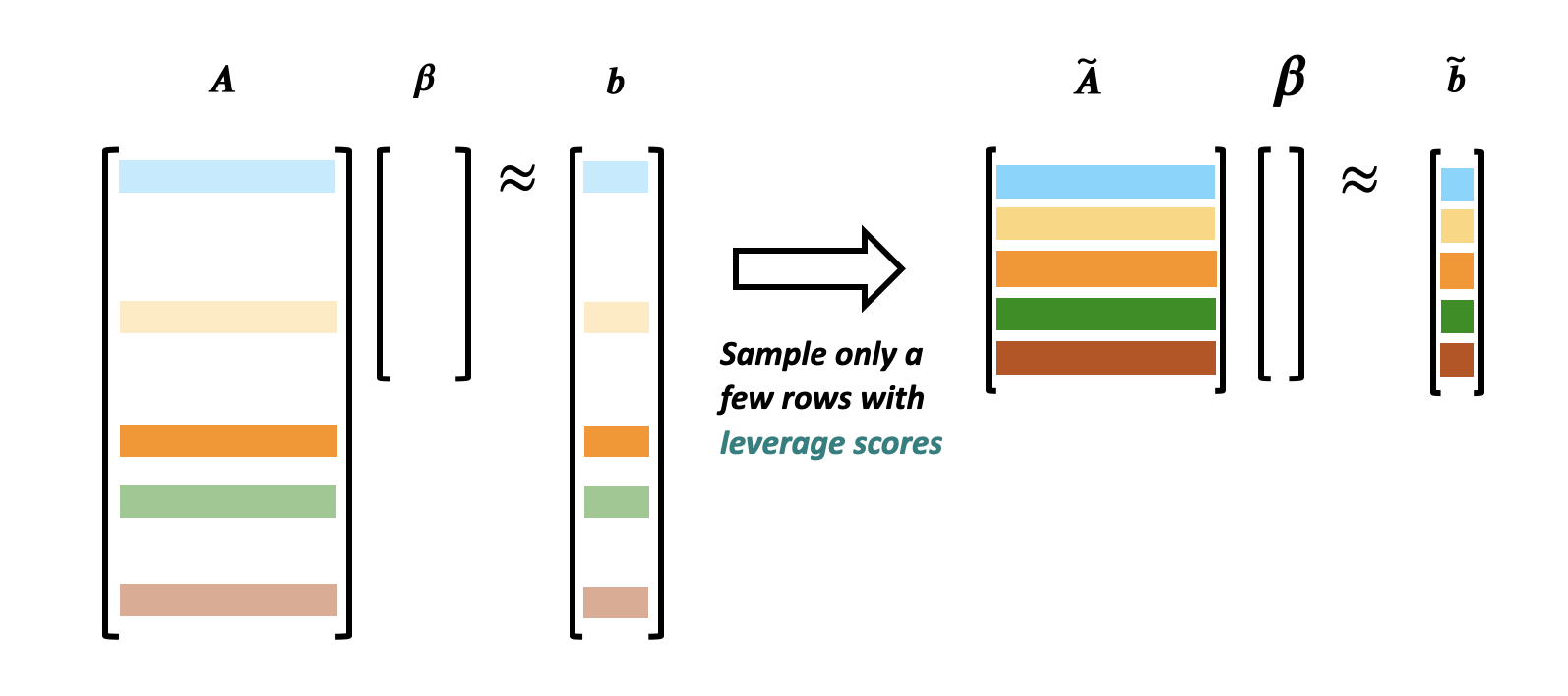
Kernel Shap works by approximating the regression using only a subset of the rows and comparing it to the corresponding subsection of the Shapley scores.
The advantage of this approach is that we are able to train a regression model while using significantly less compute since we are only computing a subset of the Shapley values, however there are some disadvantages.
The first such disadvantage is that some points are more impactful than others. Because of this our approximation may suffer if it samples a subset which is largely non-representative of the dataset, or which has an abnormal slope in a given dimension.
Key Question: How can we ensure that we are choosing a good subset of the Shapley values, without significantly increasing our time complexity?
Leverage Scores
Goals: We would like to maintain performance while getting a theoretical guarantee of accuracy.
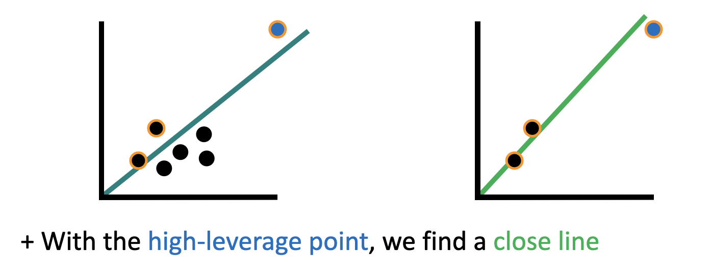
Kernel Shap attempts to approximate the linear regression, but it suffers from the fact that some points are more important than others to the preservation of the line. One approach to fix this is by assigning each point an amount of leverage based on how important it is to maintaining the slope.
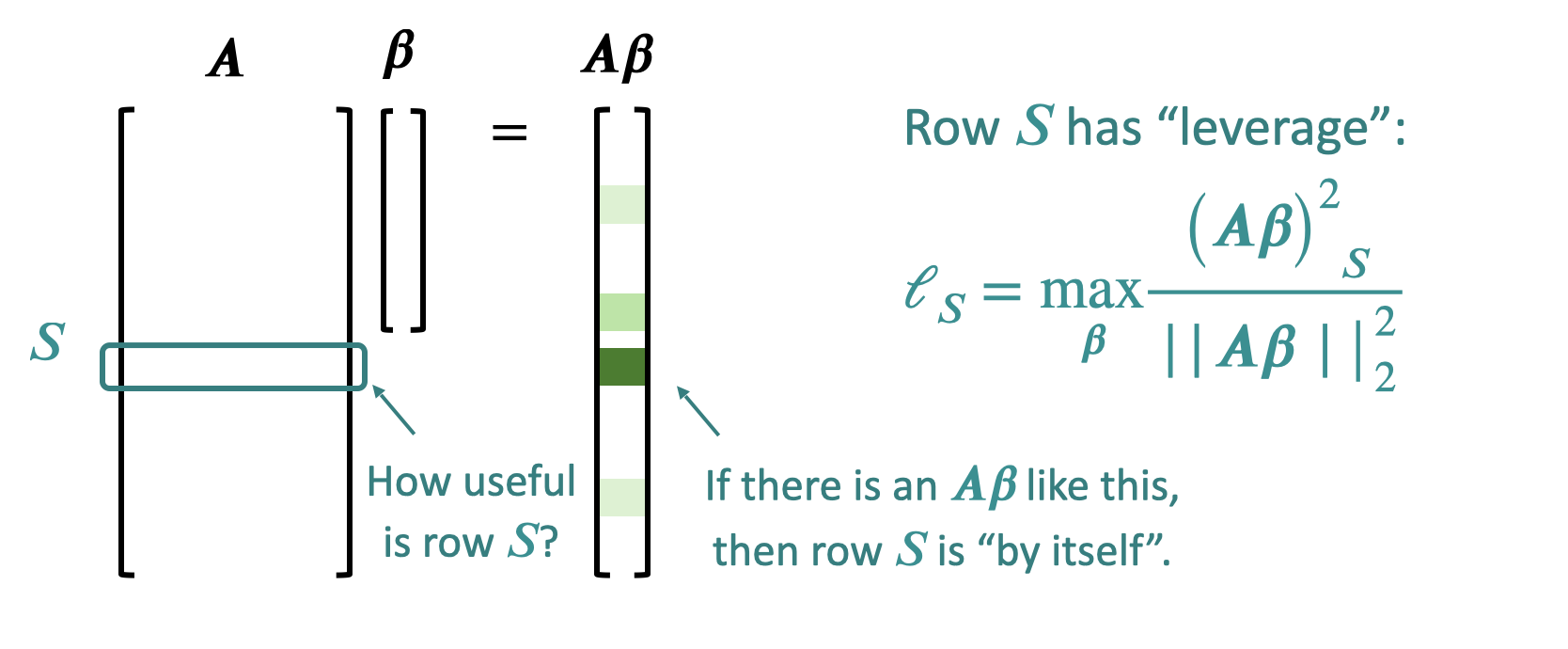
In order to calculate the leverage score of a row S, we calculate that row S has leverage:
Leverage Shap
Idea: Kernel Shap, but rather than sampling a random subset of rows, we instead sample rows proportional to their leverage score. This method results in significantly lower comparative loss than either Kernel Shap or Optimized Kernel Shap.
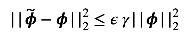
Leverage Shap comes with the additional bonus of a guarantee that if \(\gamma = \frac{\|A \phi - b\|_2^2}{\|A \phi\|_2^2}\) for all \(\epsilon \geq 0\) with \(O(nlog(n) + \frac{n}{\epsilon})\) samples and with probability \(\frac{99}{100}\).