Convolutional Neural Networks and Image Embeddings
Written by Jayda Gilyard and Josef Liem
Motivation
In class, we have already covered some useful kinds of layers that we can include in our model: fully connected layers (FCLs), attention layers, activation layers (Sigmoid, Softmax, ReLU, etc…). Today, we will talk about new kind of layer that can be used called convolution.
Why should we care about convolution when we already saw that we can perform classification using a sequence of linear layers and activations?
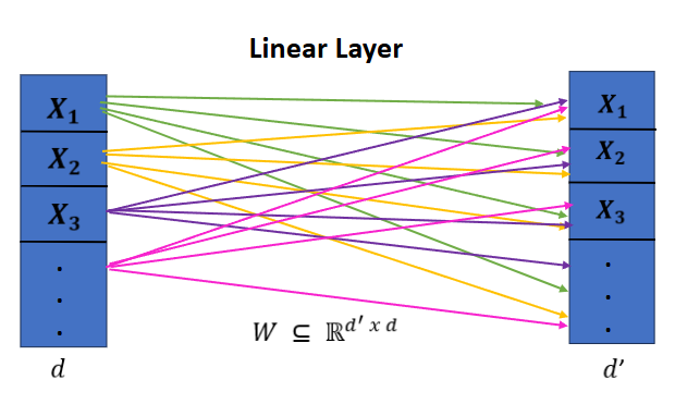
If we are interested in working with large input vectors, this will involve massive matrix multiplication with time complexity \(\theta(dd')\) where \(d\) denotes the size of the input vector, an \(d'\) the output vector. In 2D, this is particularly problematic if we wanted to build an image classifier for, say, 1024x1024 images, as we would be performing many large matrix multiplications. Thus, given that a model may consist of many linear layers, the number of trainable parameters in the model becomes far too expensive to handle at scale.
Enter Convolution…
Instead, we can take advantage of the notion of shared weights in convolution through a kernel (also called a filter), to be far more efficient. Let us first take a look at the 1-dimensional case for convolution.
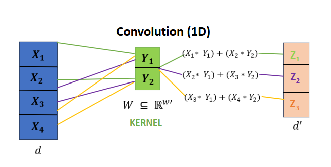
In our convolutional layer, our kernel is composed of a set of learnable weights for which we take the inner product with entries of the input vector, summing over it. We then slide this kernel over by a certain stride to generate the next scalar entry in the output vector.
More formally, where \(y\), is the result of a summation over the inner products of the input \(x\) and weights \(w\) of the kernel, we can express 1-dimensional convolution as:
\[y[n]=\sum_{i}x[i] ⋅ w[n-i]\]
In this new kind of layer, the weights in the kernel are shared with the entirety of the entries of the input, rather than defining a weight for each input/output pair, giving us complexity \(\theta(w) + \theta(d'w)\).
There are several major advantages to using convolution:
- We can use shared weights rather than having weights for each input/output entry pair.
- We can be remarkably more efficient by not performing massive matrix multiplications.
- We can take advantage of spatial locality in the input, which can be good when our data consists of sequential information. That is, in almost all images (with the exception of noise perhaps), nearby pixels are more likely to be related to each other than pixels that are far apart.
Convolution in 2 Dimensions
When we are performing convolution in machine learning, we are usually talking about 2-D convolution on images. Here, rather than a vector, our kernel now takes the form of a \(w' * w'\) matrix \(W\) which we slide over the \(d * d\) input, taking the summation over the inner product of weights and entries, producing a \(d' * d'\) output.
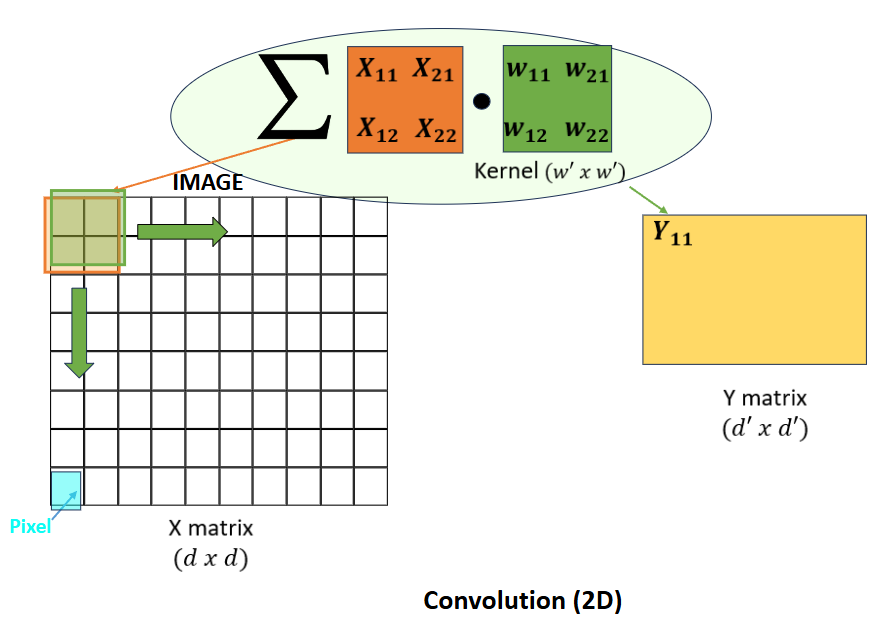
We only need to make some slight adjustments to the previous definition of 1-dimensional discrete convolution to reach 2-dimensions:
\[y[m, n]=\sum_{i}\sum_{j}x[i, j] ⋅ w[i-m, j-n]\]
- \(x[i, j]\) denotes the input at position \(i, j\).
- \(y[m, n]\) denotes the output at position \(m, n\).
- \(w[i-m, j-n]\) denotes the kernel weights with some shift over the input.
Note that the resulting shape of the output of convolution heavily depends on the shape of of \(x\), the shape of \(w\), and thus the number of strides the kernel is able to take across the input. In addition to choosing a different kernel or input shape, there are several notable modifications during convolution that will allow us to control the \(d' * d'\) shape of the output:
- Stride
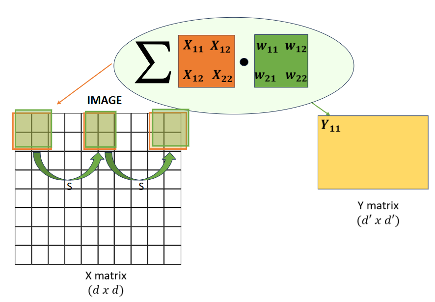
We can set our stride to be some value \(s\), such that our kernel will move by \(s\) entries when taking the summation over the inner product of input/kernel entries and weights. Increasingly large strides in convolution reduce the size of the spatial dimensions of the output.
- Padding
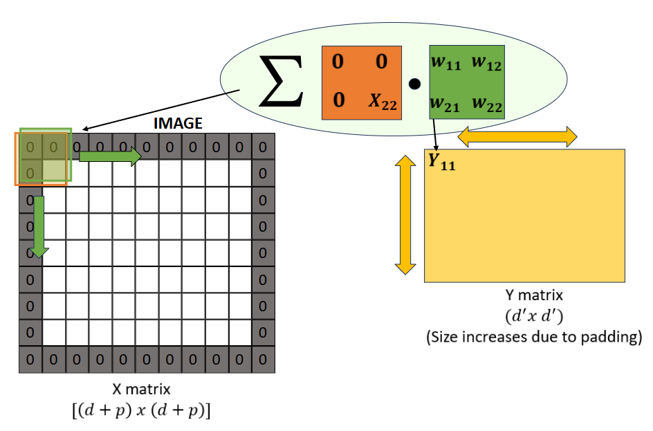
We can apply padding (usually a bunch of 0s) around our input \(x\). Adding padding will change the number of strides we might take in the given row height/column height, affecting the shape of our output.
- Dilation
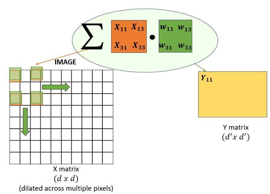
Dilation is another technique that can be applied to convolutional layers to expand the receptive field of the kernel without increasing the number of parameters.
Kernels, Features, and More…
What in an image is the kernel (hopefully) picking up on?
Ideally, in an image context, convolution is nice because kernels can pick up on features such as types of edges, corners, textures, and shapes when trying to perform classification. If we use sequences of convolutional layers, deeper layers might capture more abstract or complex features, whereas initial layers focus on more fine grained detail. Additionally, in practice, we usually apply several convolutional kernels to pick up on different kinds of features at a given layer, determining the number of output channels that the layer will produce. Many convolutional-based architectures will tend to increase the number of channels while reducing the overall spatial dimensions at subsequent layers.
Upsampling
What about upsampling?
As our previous illustrations have implicitly shown, we often talk about convolution as downsampling the original input such that the spatial dimensions gradually decrease at each convolutional layer. However, upsampling is not only possible, but often necessary in models the use an autoencoder-based architecture for image generation/reconstruction (see autoencoders next section). This is called transposed convolution or also deconvolution.
Embeddings
Autoencoders
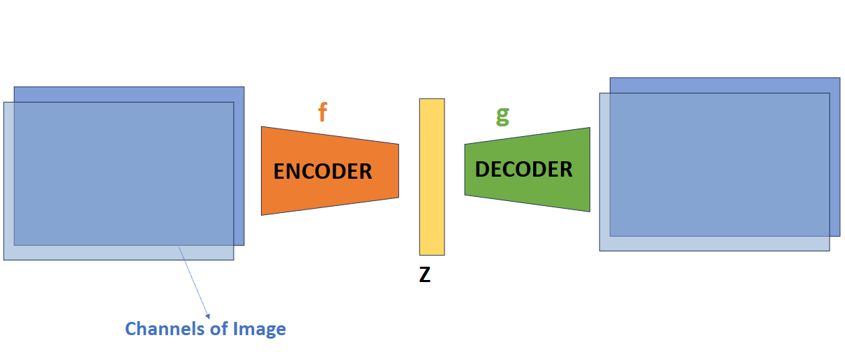
For embeddings over images, we can use an autoencoder, which consists of an encoder and a decoder. The encoder applies a set of kernels through several convolutional layers to generate a latent vector \(z\) — a compressed representation of our image. Subsequent transposed convolutions in the decoder layers can reconstruct an output image.
For the loss, instead of cross entropy, we can use mean-squared error, performed pixel-wise to look at “distance” between images:
\[L(w)=||g(f(x))-x||^2_2\]
Contrastive Learning
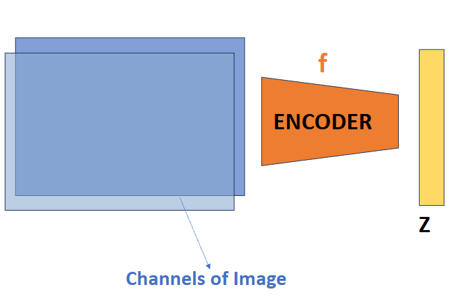
We have also seen an alternative approach - contrastive learning, that would allow us to perform initial training without the decoder. In this approach, we take positive pairs \((x, x^+)\) and negative pairs \((x, x^-)\) of images. The goal of contrastive learning is to have positive pairs end up close together in latent space and negative pairs far apart. Equivalently:
- The inner product of \(f(x)^Tf(x^+)\) should be large
- The inner product of \(f(x)^Tf(x^-)\) should be small
How do we sample positive and negative pairs of images?
- Someone manually labelled positive and negative pairs of images (supervised)
- We perform croppings on a given image and sample croppings of the same larger image are considered positive pairs, and unrelated croppings are negative
Variational Autoencoders
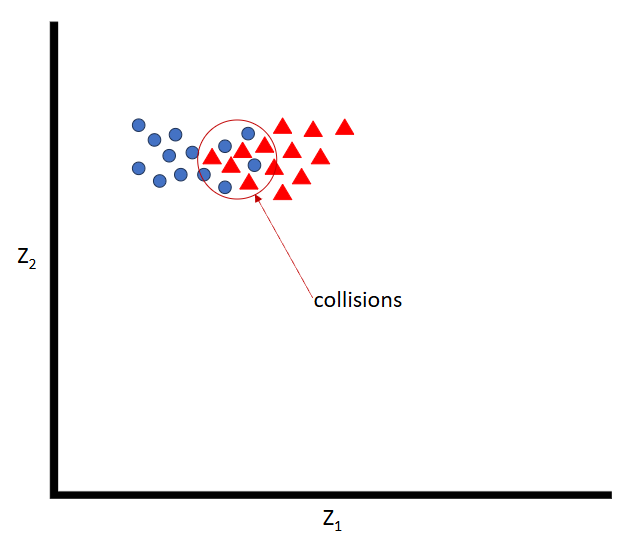
While autoencoders are a nice approach, notice that unlike contrastive learning where we try to separate negative pairs, nothing about the autoencoder forces even spacing in the latent space, allowing for potential collisions between instances of differing classes of images.
Variational autoencoders (VAEs) solve this problem probabilistically by introducing a probabilistic encoder and decoder. Instead of mapping an input to a single point in the latent space, the encoder maps the input to a distribution over the latent space. The decoder then samples from this distribution to reconstruct the input.
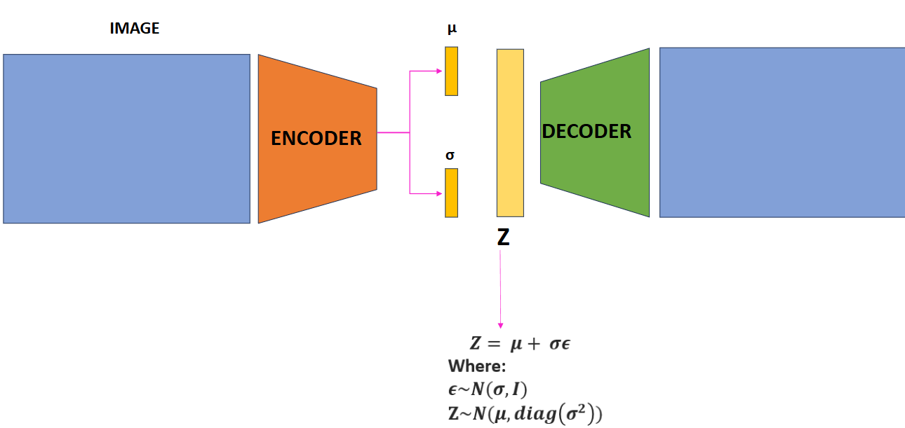
The encoder outputs the mean \(\mu\) and standard deviation \(\sigma\) of the latent distribution, and we sample a latent vector \(z\sim\mathcal{N}(\mu, \text{diag}(\sigma^2))\) from this distribution using:
\[z = \mu + \sigma \epsilon\]
where \(\epsilon\) is sampled from a Gaussian distribution \(\epsilon\sim\mathcal{N}(0, I)\).
The loss function for VAEs consists of two parts:
- Reconstruction loss: \(L_{\text{reconstruction}}=||g(f(x))-x||^2_2\). This measures how well the decoder reconstructs the input from the latent vector.
- KL divergence: \(L_{\text{variational}}=\text{dist}(\mathcal{N}(0, I), \mathcal{N}(\mu, \text{diag}(\sigma^2)))\). This measures how close the learned latent distribution is to the normal distribution.
Thus, the reconstruction is both meaningful and the latent space is evenly distributed.