Logistic Regression and Cross Entropy Loss
Written by Julian Grijalva
Motivation
In many supervised learning settings, Linear regression is not appropriate because:
The output space is discrete rather than continuous (e.g., classifying emails as spam/not spam) We need probabilities to quantify uncertainty in our predictions. Linear regression can produce values outside [0,1], making probability interpretation impossible.
Classification addresses these limitations by explicitly modeling the probability of class membership. Rather than outputting arbitrary real numbers, we want our models to output well-calibrated probabilities that can inform decision-making and risk assessment.
Supervised Binary Classification
At times, we will build models with data whose output values are discrete rather than Linear. For these cases, it is not appropriate to use Linear Regression. Instead, these models will use an approach called Supervised Binary Classification. For these such models, imagine a dataset represented as:
\(\mathcal{D} = \{(x^i, y^i)\}_{i=1}^n, \; x^i \in \mathbb{R}^d, \; y^i \in \{0, 1\}\)
Our output value y, is represented as a binary value, either 1 for ‘True’ or 0 for ‘False’.
Our end goal for this method is for our Model’s predicted output \(F(x) = \text{Output}\) to equal the predicted probability of a possitive class (binary value 1). This allows us to later optimize the model by using optimizers which reward correct and confident results, while indicating a high level of loss for confident and incorrect results.
Sigmoid Function
In the context of logistic regression, the sigmoid function is a mathematical function used to map real-valued inputs into a probability range between 0 and 1. It is defined as:
\(\sigma(z) = \frac{1}{1 + e^{-z}}\)
The sigmoid function ensures the output of logistic regression is bounded between 0 and 1, making it suitable for probabilistic interpretation.
Compared to Linear Regression, Logistic Regression Models use this sigmoid as an activation function to ensure output of a probability in the range [0,1].
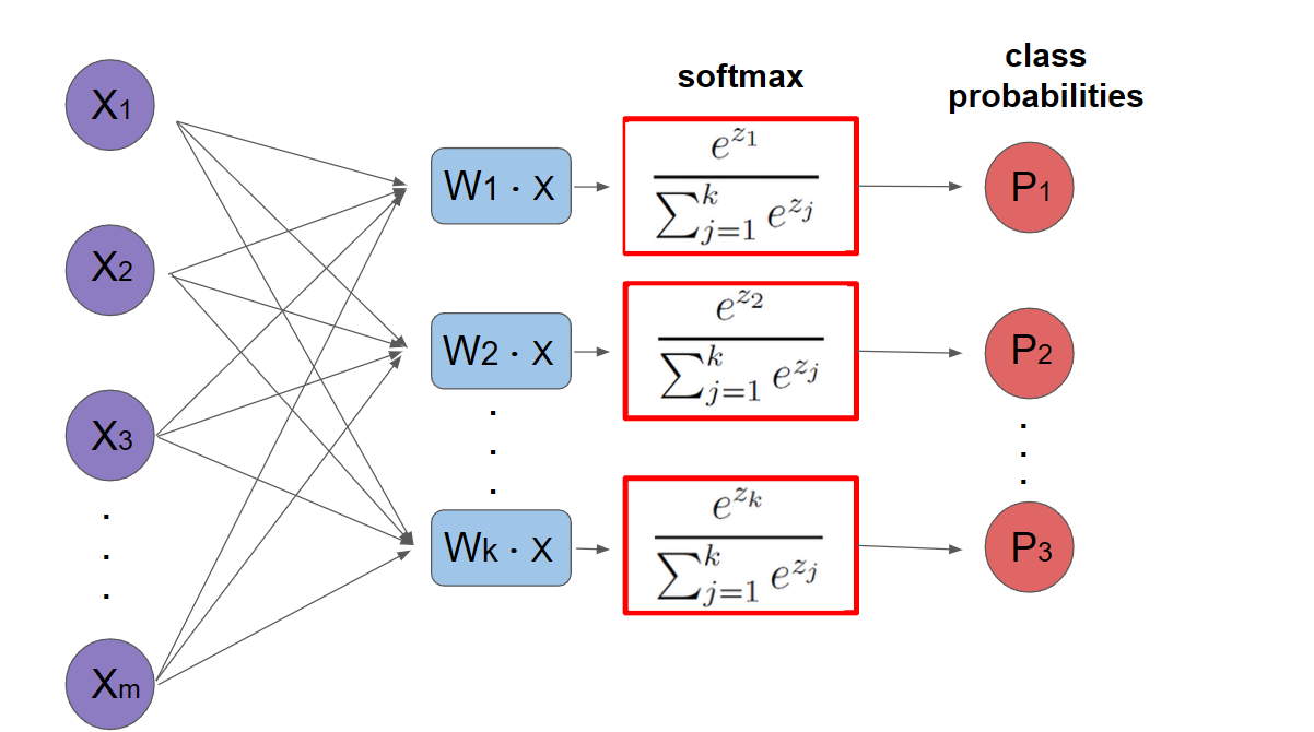
General Classification Model
When dealing with k > 2 classes, we need to output a probability distribution over all possible classes. This requires:
Multiple neurons: Each class gets its own weight vector \(w_i\) to compute class-specific scores Softmax activation: Converts raw scores into proper probabilities that sum to 1.
For input x, the model computes: \(z_i = w_i^T x + b_i\) for i = 1,…,k \(f_i(x) = \frac{e^{z_i}}{\sum_{j=1}^k e^{z_j}}\) The softmax function ensures:
All outputs are positive (due to exponential) Outputs sum to 1 (due to normalization) Preserves ordering of inputs (monotonic)
Application of softmax equation:
Cross Entropy Loss
Cross entropy provides a natural way to compare the predicted probability distribution with the true distribution encoded as one-hot vectors. For a single example with true class j: \(H(y, f(x)) = -\sum_{i=1}^k y_i \log(f_i(x)) = -\log(f_j(x))\) This loss function has important properties:
Simplifies to negative log probability of true class (since y is one-hot) Goes to infinity as predicted probability approaches 0, strongly penalizing confident wrong predictions Matches information theoretic notion of coding length Proper scoring rule (minimized by true probabilities).
The negative log function’s shape explains these properties:
Steep slope near 0 → large gradients for wrong predictions.
Shallow slope near 1 → small gradients for correct predictions.
Asymptote at 0 → infinite loss for completely wrong predictions.
binary encoding and entropy
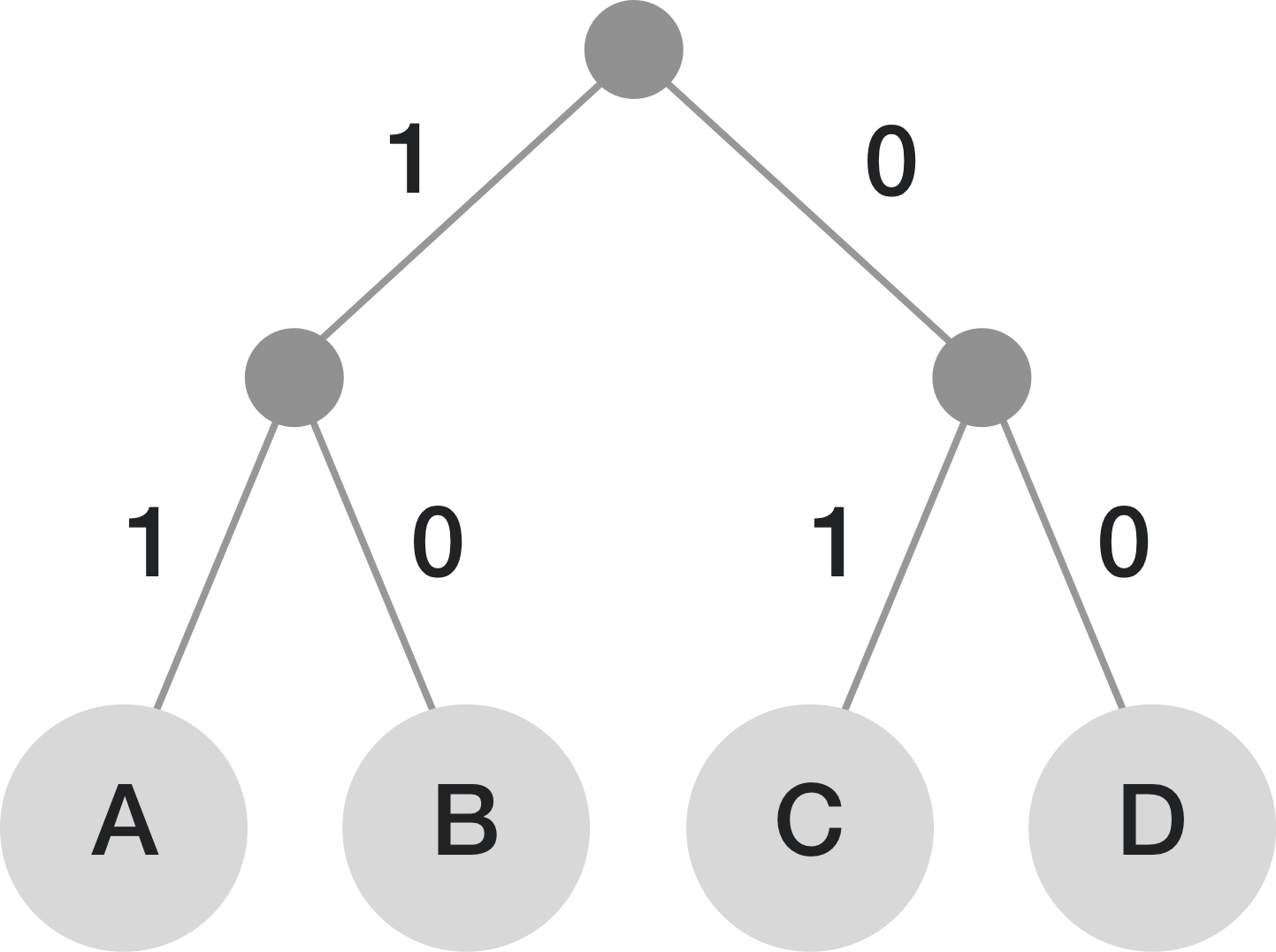
In these logistic deep learning models, discrete information must be given to the model by encoding categories using bit integer values. For example, assigning A,B,C,D to 00,01,10,11 is an example of fixed-length encoding. This is straightforward and works well when all labels are equally likely to occur. However, if the symbols are not equally likely, this approach is inefficient because it doesn’t take advantage of the differing probabilities.
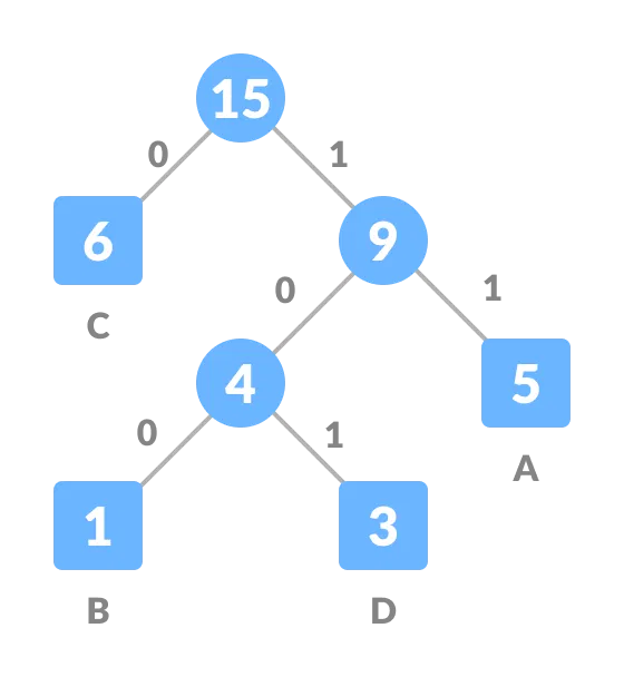
When the probability distribution of symbols is known, variable-length encoding becomes more efficient. The idea is to assign:
-Shorter codes to more common symbols. -Longer codes to less common symbols.
This minimizes the expected number of bits required to encode a sequence of symbols, leading to more efficient storage or communication.
Below are examples of fixed length encoding vs variable-length encoding for a distribution with many C’s, some A’s, and less B and D’s:
Shannon’s entropy formula quantifies the minimum average number of bits required to encode symbols from a probability distribution:
\(H(q) = -\sum_{i} p_i \log_2(p_i)\)
In order to find the entropy loss between two different distributions p and q:
\(H(p,q) = -\sum_{i} p_i \log_2(q_i)\)
Conclusion
We now have model of outputting predictions for classification and a loss. Logistic regression represents a fundamental approach to binary classification problems, distinct from linear regression by its ability to handle discrete outputs through probability estimation.
Exact computation won’t work like it did for linear regression, so we need a new strategy for this kind of problem.
The sigmoid function serves as the crucial bridge, transforming linear combinations of inputs into probabilities between 0 and 1, making it ideal for binary classification tasks.
Cross entropy loss plays a vital role in measuring model performance, providing a mathematically sound way to quantify the difference between predicted probabilities and actual binary labels. Its properties make it particularly effective for gradient descent optimization, as it heavily penalizes confident but incorrect predictions while rewarding accurate ones.
The connection to information theory through binary encoding and entropy demonstrates the broader theoretical foundation of these concepts. Whether using fixed-length or variable-length encoding, the choice of representation impacts the efficiency of information storage and processing. Shannon’s entropy formulas provide a mathematical framework for quantifying these efficiencies and measuring the divergence between probability distributions.